Schrödinger equation
| Time-dependent |
 |
| Time-independent |
 |
| Quantum mechanics |
|---|
 |
| Introduction Glossary · History |
|
Background
|
|
Fundamental concepts
|
|
Formulations
|
|
Equations
|
|
Advanced topics
|
|
Scientists
Bell · Bohm · Bohr · Born · Bose
de Broglie · Dirac · Ehrenfest Everett · Feynman · Heisenberg Jordan · Kramers · von Neumann Pauli · Planck · Schrödinger Sommerfeld · Wien · Wigner |
The Schrödinger equation was formulated in 1926 by the Austrian physicist Erwin Schrödinger. Used in physics (specifically quantum mechanics), it is an equation that describes how the quantum state of a physical system changes in time.
In classical mechanics, the equation of motion is Newton's 2nd law, and equivalent formulations are the Euler-Lagrange equations and Hamilton's equations. In all these formulations, they are used to solve for the motion of a mechanical system, and mathematically predict what the system will do at any time beyond the initial settings and configuration of the system.
In quantum mechanics, the analogue of Newton's law is Schrödinger's equation for a quantum system, usually atoms, molecules, and subatomic particles; free bound, or localized. It is not a simple algebraic equation, but (in general) a linear partial differential equation. The differential equation encases the wavefunction of the system, also called the quantum state or state vector.
In the standard interpretation of quantum mechanics, the wavefunction is the most complete description that can be given to a physical system. Solutions to Schrödinger's equation describe not only molecular, atomic, and subatomic systems, but also macroscopic systems, possibly even the whole universe.[1]
Like Newton's 2nd law, the Schrödinger equation can be mathematically transformed into other formulations such as Werner Heisenberg's matrix mechanics, and Richard Feynman's path integral formulation. Also like Newton's 2nd law, the Schrödinger equation describes time in a way that is inconvenient for relativistic theories, a problem that is not as severe in matrix mechanics and completely absent in the path integral formulation.
Contents |
Introduction - energy
To predict how a system will behave, it is useful to consider:
- The properties of the system and its constituents
- The constraints on the system, i.e. the limits of what can happen.
Analogies
For now, consider the energy of a familiar macroscopic system: a roller coaster. The roller coaster rides on a track, and is confined to it: it can travel back and forth on the track, but can't rise of it or de-rail to one side. This is one constraint of the system. For simplicity, neglect heat transfer due to friction, so the only energies associated with the roller coaster are the kinetic energy due to its motion (mass and velocity, more precisley momentum), and gravitational potential energy by virtue of height above the ground. The total energy of the system is constant - another constraint, for the coaster has a maximum amount of velocity and maximum height it can attain. The track can bend in any curved direction. At a peak in the track, the roller coaster exchanges kinetic energy into gravitational potential energy to climb over the peak, doing work against gravity. Near a dip in the track, the roller coaster transfers its potential energy into kinetic energy as it falls down towards the base of the dip. The coaster can pass over the next peak if it has enough energy, if not then it will reverse direction and fall back into the well, and then rise up the slightly, then fall back down again. Since there are no losses due to friction, the coaster will fall and rise to the same height. The reversal of direction is due to the alternating kinetic and potential energy exchange.
In quantum mechanics, a sub-atomic particle is like the roller coaster, confined to some region of space (like dips of track) or is free (if the coaster is racing along the track), and can exchange kinetic energy and potential energy in a similar way. Sometimes the particle is confined to a region due to the potential energy exceeding the kinetic energy of the particle. This is the principle behind electrons in atoms: they are bounded an electrostatic potential. [2].
Another analogy is a ball thrown at a wall - it will never penetrate it because it doesn't have enough energy. This is energy transfer on the macroscopic scale. At the microscopic scale, a particle "bouncing" in a constant-potential well (potential energy is finite) can penetrate the barrier and pass through, if its energy is greater than the potential, though only by chance. The whole situation is described by solutions to the time-independent Schrödinger equation for the situation (see below for details of this instance). The chance of a particle doing something, at some place, is the wavefunction.
The idea of constraints using energies is used in the set-up of the Schrödinger equation, for particles at the atomic and sub-atomic scale.
Application
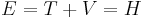
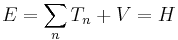
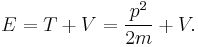
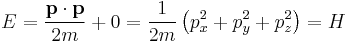
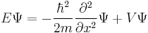
Consider the total energy of a quantum system, constituting a particle subject to a potential (say an electric potential due to an electric field). The total energy of the system can be split into the sum of two parts: the kinetic energy of the particle due to its motion (mathematically a function of velocity, or alternatively momentum), and potential energy due to its position (a function of spatial coordinates, and possibly time). The potential energy of the particle corresponds to the type of potential in the system. This can be translated into an extremely simple equation:

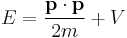
where T is the kinetic energy and V is the potential energy of the particle, E is the total energy. The sum of the kinetic energy and potential energy is known as the Hamiltonian function (a function of position - due to the potential energy, and velocity - due to kinetic energy), so
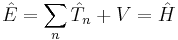
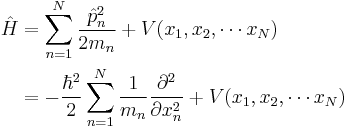
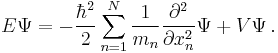
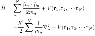
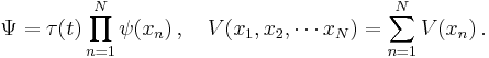
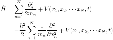
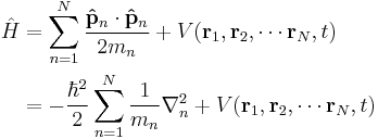
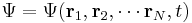
This formalism can be extended to any number of particles: the total energy of the system, also the Hamiltonian, is then the sum of the kinetic energies of the particles, plus the total potential energy. Mathematically, again its a very simple sum:
where the sum is taken over all the particles in the system. However, there can be interactions between the particles (an N-body problem), so the potential energy V can change as the spatial configuration of particles changes, and possibly with time. The potential energy, in general, is not the sum of the separate potential energies for each particle, it is a function of all the spatial positions of the particles.
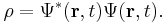
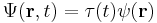
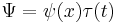
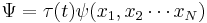
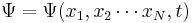
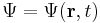
The wavefunction, denoted Ψ, summarizes the quantum state of the particles in the system, limited by the constraints on the system: the probability the particles are in some spatial configuration at some instant of time.
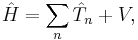
One of the postulates of quantum mechanics is that all observables are represented by operators which act on the wavefunction, so in the previous equations the energies of the particle are replaced by their operator equivalents:
where the circumflexes ("hats") denote operators. The energy operators are mostly differential operators, except for potential energy V, which is just a multiplicative factor.
Collecting these ideas together, it should be possible to structure an equation based on the energies of the particles - their possible kinetic and potential energies the system constrains them to have, in terms of the state of the system, and solve it for the wavefunction. Casting the operators and wavefunction together yields a differential equation of the wavefunction: The Schrödinger equation. The result is that the Schrödinger equation is a differential equation of the wavefunction, and solving it for the wavefunction can be used to predict how the particles will behave under the influence of the specified potential and with each other. The form of the Schrödinger equation depends on the physical situation (see below for special cases).
Equation
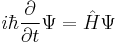
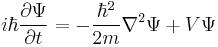
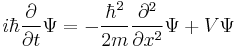
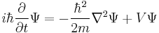
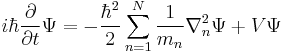
The most general form is the time-dependent Schrödinger equation, which gives a description of a system evolving with time,[3] more fully and more useful:
where Ψ is the wave function of the quantum system,

is the energy operator (i is the imaginary unit and ħ is the reduced Planck constant), and  is the Hamiltonian operator, the form of which depends on the system.
In its most general form,
where the sum is taken over all of the particles;
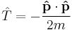
is the kinetic energy operator with m being the mass of particle; and

is the momentum operator, and ∇ is the gradient operator (del).
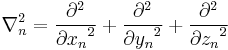
By cumulative substitution, the Hamiltonian used in the Schrödinger equation is
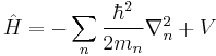
∇n is the gradient operator for the spatial coordinates of particle n, see below for details.
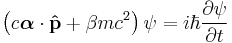
Care must be taken in which equation to actually name "the Schrödinger equation". Interestingly, the boxed equation is also true in relativistic quantum mechanics, but very frequently this equation is still referred to as the Schrödinger equation. When the form of the Hamiltonian, as given above, is used, it is still without mistake called the Schrödinger equation. However if a different Hamiltonian was used, such as
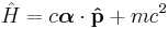
the boxed equation becomes the Dirac equation. What defines the Schrödinger equation is the classical expressions for the Hamiltonian, and this is the barrier between the "Schrödinger equation" and relativity. The classical equations are only the low-velocity limit of relativity.
To use Schrödinger equation, the Hamiltonian operator is set up for the system, accounting for the kinetic and potential energy of the particles constituting the system, then inserted into the Schrödinger equation. The resulting partial differential equation is solved for the wavefunction, which contains information about the system.
For systems in a stationary state, that is when the Hamiltonian is not dependent on time, time-dependence of the equation reduces only spatial dependence,; this form of the equation is the time-independent Schrödinger equation. In all other instances, the full time-dependent equation must be used.
The equation can be solved exactly for a few idealized cases, but is not soluble for most practical situations. For example, to analyse the behaviour of electrons in atoms, i.e. the probability the electrons are at a given point in space and time, approximate methods are needed to solve the equation.
In practice, in particular research in particle physics, high-energy physics, and quantum chemistry, physicists use natural units to simplify calculations with the equation. There are many systems of natural units, particle physicists may use Planck units or the natural system developed for particle physics, while quantum chemists use Atomic units, in each case ħ = 1. This article does not use natural units, since SI units are simpler to follow by dimensional analysis, although further implications of natural units are discussed below, relevant to wave-particle duality.
Historical background and development
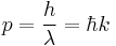
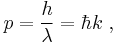
Following Max Planck's quantization of light (see black body radiation), Albert Einstein interpreted Planck's quanta to be photons, particles of light, and proposed that the energy of a photon is proportional to its frequency, one of the first signs of wave–particle duality. Since energy and momentum are related in the same way as frequency and wavenumber in special relativity, it followed that the momentum p of a photon is proportional to its wavenumber k.
Louis de Broglie hypothesized that this is true for all particles, even particles such as electrons. He showed that, assuming that the matter waves propagate along with their particle counterparts, electrons form standing waves, meaning that only certain discrete rotational frequencies about the nucleus of an atom are allowed. These quantized orbits correspond to discrete energy levels, which reproduced the old quantum condition.[4]
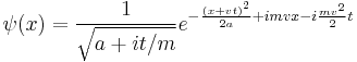
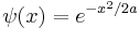
Following up on these ideas, Schrödinger decided to find a proper wave equation for the electron. He was guided by William R. Hamilton's analogy between mechanics and optics, encoded in the observation that the zero-wavelength limit of optics resembles a mechanical system — the trajectories of light rays become sharp tracks that obey Fermat's principle, an analog of the principle of least action.[5] A modern version of his reasoning is reproduced below. The equation he found is:[6]
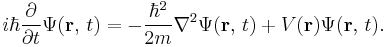
Using this equation, Schrödinger computed the hydrogen spectral series by treating a hydrogen atom's electron as a wave Ψ(x, t), moving in a potential well V, created by the proton. This computation accurately reproduced the energy levels of the Bohr model. In a paper, Schrödinger himself explained this equation as follows: "The already ... mentioned psi-function.... is now the means for predicting probability of measurement results. In it is embodied the momentarily attained sum of theoretically based future expectation, somewhat as laid down in a catalog." [7]
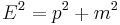
However, by that time, Arnold Sommerfeld had refined the Bohr model with relativistic corrections.[8][9] Schrödinger used the relativistic energy momentum relation to find what is now known as the Klein–Gordon equation in a Coulomb potential (in natural units):
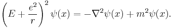
He found the standing waves of this relativistic equation, but the relativistic corrections disagreed with Sommerfeld's formula. Discouraged, he put away his calculations and secluded himself in an isolated mountain cabin with a lover.[10]
While at the cabin, Schrödinger decided that his earlier non-relativistic calculations were novel enough to publish, and decided to leave off the problem of relativistic corrections for the future. He put together his wave equation and the spectral analysis of hydrogen in a paper in 1926.[11] The paper was enthusiastically endorsed by Einstein, who saw the matter-waves as an intuitive depiction of nature, as opposed to Heisenberg's matrix mechanics, which he considered overly formal.[12]
The Schrödinger equation details the behaviour of ψ but says nothing of its nature. Schrödinger tried to interpret it as a charge density in his fourth paper, but he was unsuccessful.[13] In 1926, just a few days after Schrödinger's fourth and final paper was published, Max Born successfully interpreted ψ as a quantity related to the probability amplitude, which is equal to the squared magnitude of ψ.[14] Schrödinger, though, always opposed a statistical or probabilistic approach, with its associated discontinuities—much like Einstein, who believed that quantum mechanics was a statistical approximation to an underlying deterministic theory— and never reconciled with the Copenhagen interpretation.[15]
The wave equation for particles
The Schrödinger's equation was developed principally from the De Broglie hypothesis, a wave equation that would describe particles[16], and can be constructed in the following way.[17] For a more rigourous mathematical derivation of Schrödinger's equation, see also [18].
Assumptions
- The total energy E of a particle is the sum of kinetic energy T and potential energy V (energy conservation), for one dimension:
This is the classical expression for a particle with mass m, momentum p and total energy E. The potential energy V can vary with position, and time. This is also the frequent expression for the Hamiltonian H in classical mechanics, so E = H. For three dimensions:
where p is the momentum vector.
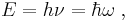
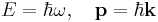
- Einstein's light quanta hypothesis (1905) assert that the energy E of a photon is proportional to the frequency ν (or angular frequency, ω = 2πν) of the corresponding electromagnetic wave:
- The de Broglie hypothesis (1924) states that any particle can be associated with a wave, and that the momentum p of the particle is related to the wavelength λ of such a wave, in one dimension, by the equation:
In three dimensions de Broglie's equation is
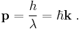
where k is the wavevector (wavelength is related to the magnitude of k)
- The previous assumptions only allows one to derive the equation for plane waves, corresponding to free particles. Other physical situations are not purely described by plane waves. So to conclude that it is true in general requires the superposition principle; any wave can be made by superposition of sinusoidal plane waves. So if the equation is linear, a linear combination of plane waves is also an allowed solution. Hence a necessary and separate requirement is that the Schrödinger equation is a linear differential equation.
Derivation from plane waves
The Schrödinger equation is mathematically a wave equation, since the solutions are at least plane waves, or linear combinations of them. However, the framework to the equation is the energy of the particle. The connection between the Schrödinger equation and wave-particle duality, mathematically, may be understood as follows.
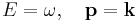
The Planck-Einstein and De Broglie relations
illuminate the deep connections between space with momentum, and energy with time. This is more apparent using natural units, setting ħ = 1 makes these equations into identities:
Energy and angular frequency both have the same dimensions as the reciprocal of time, and momentum and wavenumber both have the dimensions of inverse length. These may be used interchangeably, and in practice they normally are (at a post-graduate level and in theoretical physics research). A more interesting point is that energy is also a symmetry with respect to time, and momentum is a symmetry with respect to space, and these are the reasons why energy and momentum are conserved - see Noether's theorem. However, we continue to use SI units for familiarity.
Schrödinger's great insight, late in 1925, was to express the phase of a plane wave as a complex phase factor:

and to realize that the first order partial derivatives with respect to space
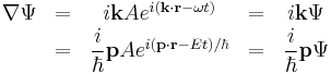
and time
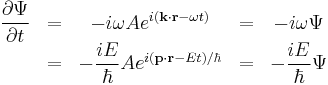
yeild the relations
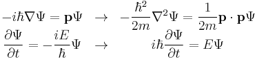
The dimensions between energy and time, and momentum and wavenumber, can be seen to match again. Multiplying the energy equation by Ψ
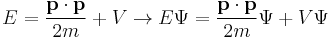
immediately lead Schrödinger to his equation:
The previous derivatives also lead to the energy operator, corresponding to the time derivative,

and the momentum operator, corresponding to the spatial derivatives (the gradient),
Substitution of these operators in the energy equation and multiplcation by Ψ yeilds the same wave equation.
Given the derivatives, wave-particle duality can be assessed as follows. The kinetic energy T is related to the square of momentum p, and hence the magnitude of the second spatial derivatives, so the kinetic energy is also proporional to the magnitude of the curvature of the wave. As the particle's momentum increases, the kinetic energy increases more rapidly, but the since the wavenumber k increases the wavelength  decreases, mathematically
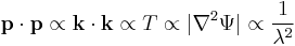
As the curvature increases, the amplitude of the wave alternates between positive and negative more rapidly, and also shortens the wavelength. So the inverse relation between momentum and wavelength is consistent with the energy the particle has, and so the energy of the particle has a connection to a wave, all in the same mathematical formulation.[19]
To summarize, wave-particle duality is internal to the Schrödinger equation, and was the first equation of its type: a wave equation whose solutions describes particles.
Implications
The solutions to Schrödinger equation can correctly account for the phenomena of energy levels in atoms and molecules (see time-independent equation below), and diffraction, interference and propagation of waves and particles.
A sufficient number of plane waves can superimpose to form any wave. Although these wavefunctions are not "real", in the sense that they are complex valued functions which serve as convenient mathematical constructs, and can't be observed, the mathematics (using imaginative thought experiments) can still continue to describe them as though they really are real waves (water, mechanical or electromagnetic). Schrödinger for one studied the philosophy of what wavefunctions actually mean in nature, just as much as he deduced them mathematically (see interpretations of quantum mechanics).
These waves can reflect from boundaries due to potentials, and set up standing waves (stationary states, see below). Macroscopically, standing waves never penetrate the boundaries, but microscopically the Schrödinger equation makes it an inevitable result that waves can tunnel through barriers into classically forbidden regions.
They can also diffract and interfere, the chance of finding a particle is not fully localized towards one point, it could in a number of different places at the same time. To see this, consider some following modifications of the double-slit experiment, the diffraction effect through two apertures, close together. It can applies to particles, mechanical and luminal waves. For further details, see Feynman, 1965[20].
If a gun fired at a pair of apertures (large eneogh to let pellets through), they would miss or scatter randomly through them. Probabilities must be used, since there is no way to tell exactly where a pellet would go. The scattering of pellets everywhere is random. If waves are generated in a ripple tank of water, directed through the immersed pair of apertures, this time its easier to know where the maxima and minima would occur, since the wave fronts propagate at definite frequencies and velocities. The interference of waves is deterministic. However, using an electron gun instead of the usual type, the particles still scatter everywhere but there are so many streaming from the gun that they appear to be a continuous wave diffracting. This applies to light also.
The conclusion is that elementary particles are an effective continuum macroscopically, and the observed result is wave-like diffraction, even though the particle scattering is random. Classically, particles cannot execute any of these effects, but the Schrödinger equation allows this, and these effects of real particles are observed in experiment - and are actually used.
An electron beam can be "refracted" and "focused" by magnetic lenses[21], analogous to light refracted by glass or plastic lenses, this application is known as "electron optics", and is utilized in the electron microscope, an essential research tool.
Neutrons can also be diffracted in crystals, and is a technique used to determine their structure. Neutrons are substantially more massive than electrons, and recently an extremely small gravitational potential term in the Schrödinger equation for neutrons has been observed, in extremely sensitive experiments involving neutrons "fall under gravity". [22][23][24].
Properties
The Schrödinger equation has the following properties: some are useful, but there are shortcomings.
Linearity
If two wave functions ψ1 and ψ2 are solutions, then so is any linear combination of the two:

where a and b are any complex numbers. The sum can be extended for any number of wavefunctions. This property allows superpositions of quantum states to be solutions of the Schrödinger equation. In particular a given solution can be multiplied by any complex number. This allows one to solve for a wave function without normalizing it first.
Real energy eigenstates
The time-independent equation is also linear, with an additional featutre: if two wave functions ψ1 and ψ2 are solutions to the time-independent equation with the same energy E, then so is any linear combination:

Two different solutions with the same energy are called degenerate.[25]
In an arbitrary potential, there is one degeneracy: if a wave function ψ solves the time-independent equation, so does its complex conjugate ψ*. By taking linear combinations, the real and imaginary parts of ψ are each solutions. Thus, the time-independent eigenvalue problem can be restricted to real-valued wave functions.
In the time-dependent equation, complex conjugate waves move in opposite directions. If Ψ(x, t) is one solution, then so is Ψ(x, –t). The symmetry of complex conjugation is called time-reversal symmetry.
Local conservation of probability
The probability density ρ (probability per unit volume) and probability current j (flow per unit area) of a particle are respectivley defined as:[26]
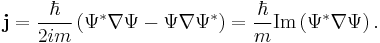
These quantities satisfy the continuity equation:
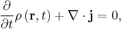
This equation is the mathematical equivalent of the probability conservation law, and can be derived from the Schrödinger equation. [27]
For a plane wave propagating in space:
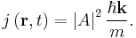
This is just the square of the amplitude of the wave times the particle's speed,
 .
.
The probability current is nonzero, even though

everywhere (that is, plane waves are stationary states). This demonstrates that a particle may be in motion even if its spatial probability density has no explicit time dependence.
Group velocity
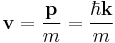
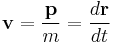
For wave motion in 3d space, Schrödinger required that a wave packet (not a plane wave) at position r with wavevector k will move along the trajectory determined by Newton's laws in the limit that the wavelength is small, i.e. for a large k and therefore large p. Consider the case without a potential, V = 0:
in which case a wavepacket should travel in a straight line at the classical velocity. The components of the group velocity v of a wavepacket are: [28][29]
![v_x = {\partial \omega \over \partial k_x } = {\partial (E/\hbar) \over \partial (p_x/\hbar)} = {\partial H \over \partial p_x} = {\partial \over \partial p_x} \left[\frac{1}{2m}\left(p_x^2 %2B p_y^2 %2B p_z^2\right) \right]= \frac{p_x}{m} = {dx \over dt}](/2012-wikipedia_en_all_nopic_01_2012/I/c3b6333147c070f5371781b07fd15727.png)
simalarly for the y and z directions, so the group velocity is
so the group velocity of the wave equals the velocity of the particle.
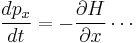
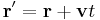
In addition, Hamilton's equations can be read off (same as in Hamiltonian mechanics):
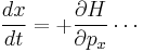
(same for the y and z directions). The group-velocity relation applied to the fourier transform of the wave-packet gives the second of Hamilton's equations,
Hamilton's equations can mathematically transform to Newton's 2nd law.
Correspondence principle
Due to the Hamiltonian in the Schrödinger equation, it satisfies the correspondence principle: in the limit of small wavelength wave packets, it reproduces Newton's laws (as stated above). This is easy to see from the equivalence to matrix mechanics. All operators in Heisenberg's formalism obey the quantum mechanics analogue of Hamilton's equations:[30]
![i\hbar{d\hat{A} \over dt} = [\hat{A},\hat{H}]= -i\hbar (\hat{A}\hat{H} - \hat{H}\hat{A})](/2012-wikipedia_en_all_nopic_01_2012/I/649e067ab6610ac3474782ed9407269f.png)
where the square brackets [ , ] denote the commutator. So, the equations of motion for the position operator  and momentum operators are the velocity: [31]

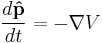
and force (same as a potential gradient):
In the Schrödinger picture, the interpretation of the above equation is that it gives the time rate of change of the matrix element between two states, when the states change with time. Taking the expectation value in any state shows that Newton's laws hold not only on average, but exactly, for the quantities:


where the integrals are taken over all space, and dr3 is a differential volume element, in cartesian coordinates dxdydz.
Positivity of energy
If the potential is bounded from below, meaning there is a minumum value of potential energy, the eigenfunctions of the Schrödinger equation have energy which is also bounded from below. This can be seen most easily by using the variational principle, as follows. (See also below).
For any linear operator  bounded from below, the eigenvector with the smallest eigenvalue is the vector ψ that minimizes the quantity

over all ψ which are normalized.[32] In this way, the smallest eigenvalue is expressed through the variational principle. For the Schrödinger Hamiltonian bounded from below, the smallest eigenvalue is called the ground state energy. That energy is the minimum value of
![\langle \psi|\hat{H}|\psi\rangle = \int \psi^*(\bold{r}) \left[ - \frac{\hbar^2}{2m} \nabla^2\psi(\bold{r}) %2B V(\bold{r})\psi(\bold{r})\right] d^3\bold{r} = \int \left[ \frac{\hbar^2}{2m}|\nabla\psi|^2 %2B V(\bold{r}) |\psi|^2 \right] d^3\bold{r}](/2012-wikipedia_en_all_nopic_01_2012/I/936ec60d380856254e8cda3ef916f83b.png)
(using integration by parts). Due to the absolute values of ψ, the right hand side always greater than the lowest value of V(x). In particular, the ground state energy is positive when V(x) is everywhere positive.
Galilean and Lorentz invariance
Galilean transformations (or "boosts") look at the system from the point of view of an observer moving with a steady velocity –v. A boost must change the physical properties of a wavepacket in the same way as in classical mechanics: [33]
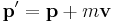
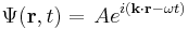
The phase factor

of a free-particle Schrödinger plane wave

threrefore transforms according to
![\begin{align} \bold{k}\cdot\bold{r} - \omega t & = (\bold{p}\cdot\bold{r} - E t)/\hbar \\
& = \left[(\bold{p}' - m\bold{v})\cdot(\bold{r}' - \bold{v}t) - (\bold{p}'-m\bold{v})\cdot(\bold{p}'-m\bold{v})t/2m \right]\hbar \\
& = \left[\bold{p}' \cdot\bold{r}' %2B E' t %2B m \bold{v} \cdot (\bold{r} - \bold{v}t/2) \right]/\hbar \\
\end{align}](/2012-wikipedia_en_all_nopic_01_2012/I/8c39cabf29b3671e0ec7ebdd43ef2b59.png)
The wavefunction therefore transforms according to

This additional terms in the phase factor imply the Schrödinger equation is not Galilean invariant: the plane wave solutions to do not remain in the same form under Galilean transformations. The transformation of an arbitrary superposition of plane wave solutions - with different values of p and E, is still the same superposition of boosted plane waves multiplied by the phase factor:

The transformation of any solution to the free-particle Schrödinger equation, Ψ(r, t) results in other solutions:

For example, the transformation of a constant wavefunction results in a plane-wave.
For another example, boosting the spreading Gaussian wavepacket:
produces the moving Gaussian:
which spreads in the same way.
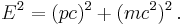
The Lorentz transformations are simalar to the Galilean ones, so the Schrödinger equation is not Lorentz invariant either, in turn not consistent with special relativity. This also can be seen from the following arguments:
Firstly, the equation requires the particles to be the same type, and the number of particles in the system to be constant, since their masses are constants in the equation (kinetic energy terms).[34] This alone means the Schrödinger equation is not compatible with relativity - even the simple equation

allows (in high-energy processes) particles of matter to completely transform into energy by particle-antiparticle annihilation, and enough energy can re-create other particle-antiparticle pairs. So the number of particles and types of particles is not necessarily fixed. For all other intrinsic properties of the particles which may enter the potential function, including mass (such as the harmonic oscillator) and charge (such as electrons in atoms), which will also be constants in the equation, the same problem follows.
Secondly, as shown above in the plausibility argument - the Schrödinger equation was constructed from classical energy conservation rather than the relativistic mass–energy relation
Finally, changing inertial reference frames requires a transformation of the wavefunction analogous to requiring gauge invariance. This transformation introduces a phase factor that is normally ignored as non-physical, but has application in some problems.[35]
Special cases
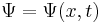
Following are several forms of Schrödinger's equation for different situations: time independance and dependance, one and three spatial dimensions, and one and N particles. In actuality, the particles constituting the system do not have the numerical labels used in theory. The language of mathematics forces us to label the positions of particles one way or another, otherwise there would be confusion between symbols representing which variables are for which particle.[18]
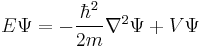
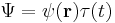
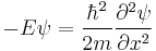
Time independent
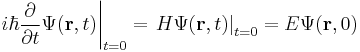
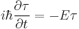
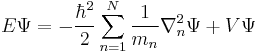
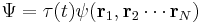
If the Hamiltonian is not an explicit function of time, the equation is separable into its spatial and temporal parts. Hence the energy operator 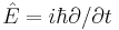 can then be replaced by the energy eigenvalue E. In abstract form, it is an eigenvalue equation for the Hamiltonian [36]

A solution of the time independent equation is called an energy eigenstate with energy E. [37]
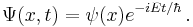
To find the time dependence of the state, consider starting the time-dependent equation with an initial condition ψ(r). The time derivative at t = 0 is everywhere proportional to the value:
So initially the whole function just gets rescaled, and it maintains the property that its time derivative is proportional to itself, so for all times t,
substituting for Ψ:
where the ψ(r) cancels, so the solution of the time-dependent equation with this initial condition is:

This case describes the standing wave solutions of the time-dependent equation, which are the states with definite energy (instead of a probability distribution of different energies). In physics, these standing waves are called "stationary states" or "energy eigenstates"; in chemistry they are called "atomic orbitals" or "molecular orbitals". Superpositions of energy eigenstates change their properties according to the relative phases between the energy levels.
The energy eigenvalues from this equation form a discrete spectrum of values, so mathematically energy must be quantized. More specifically, the energy Eigen states form a basis - any wavefunction may be written as a sum over the discrete energy states or an integral over continuous energy states, or more generally as an integral over a measure. This is the spectral theorem in mathematics, and in a finite state space it is just a statement of the completeness of the eigenvectors of a Hermitian matrix.
In the case of atoms and molecules, it turns out in spectroscopy that the discrete spectral lines of atoms is evidence that energy is indeed physically quantized in atoms; specifically there are energy levels in atoms, associated with the atomic or molecular orbitals of the electrons (the stationary states, wavefunctions). The spectral lines observed are definite frequencies of light, corresponding to definite energies, by the Plank-Einstein relation and De Broglie relations (above). However, it is not the absolute value of the energy level, but the difference between them, which produces the observed frequencies, due to electronic transitions within the atom emitting/absorbing photons of light.
Hamiltonians
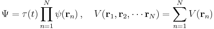
Summarized below are the various forms the Hamiltonian takes, with the corresponding Schrödinger equations and forms of wavefunction solutions.
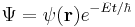
| One particle | N particles | |
| One dimension | 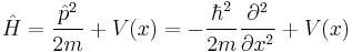 |
where the position of particle n is xn. |
 |
 |
|
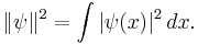
In fact the wavefunction is
There is a further restriction — the solution must not grow at infinity, so that it has either a finite L2-norm (if it is a bound state) or a slowly diverging norm (if it is part of a continuum):[38]
|
for non-interacting particles
|
|
| Three dimensions | 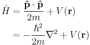
where the position of the particle is r = (x, y, z). |
where the position of particle n is r n = (xn, yn, zn), and the Laplacian for particle n using the corresponding position coordinates is
|
 |
 |
|
again more specifically:[6]
|
for non-interacting particles
|
Following are examples where exact solutions are known. See the main articles for further details.
One-dimensional examples
Free particle
For no potential, V = 0, so the particle is free and the equation reads:[39]
which has oscillatory solutions for E > 0 (the Cn are arbitrary constants):

and exponential solutions for E < 0

The exponentially growing solutions have an infinite norm, and are not physical. They are not allowed in a finite volume with periodic or fixed boundary conditions.
Constant potential
For a constant potential, V = V0, the solution is oscillatory for E > V0 and exponential for E < V0, corresponding to energies that are allowed or disallowed in classical mechanics. Oscillatory solutions have a classically allowed energy and correspond to actual classical motions, while the exponential solutions have a disallowed energy and describe a small amount of quantum bleeding into the classically disallowed region, due to quantum tunneling. If the potential V0 grows at infinity, the motion is classically confined to a finite region, which means that in quantum mechanics every solution becomes an exponential far enough away. The condition that the exponential is decreasing restricts the energy levels to a discrete set, called the allowed energies.[40]
Harmonic oscillator
The Schrödinger equation for this situation is
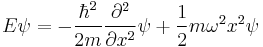
It is a notable quantum system to solve for; since the solutions are exact (but complicated - in terms of Hermite polynomials), and it can describe or at least approximate a wide variety of other systems, including vibrating atoms, molecules,[41] and atoms or ions in lattices,[42] and approximating other potentials near equilibrium points. It is also the basis of perturbation methods in quantum mechanics.
There is a family of solutions - in the position basis they are
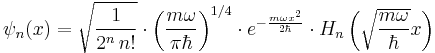
where n = 0,1,2... , and the functions Hn are the Hermite polynomials.
Three-dimensional examples
Hydrogen atom
This form of the Schrödinger equation can be applied to the Hydrogen atom:[43][44]
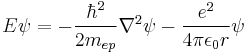
where e is the electron charge, r is the position of the electron (r = |r| is the magnitude of the position), the potential term is due to the coloumb interaction, wherein ε0 is the electric constant (permittivity of free space) and
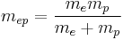
is the 2-body reduced mass of the Hydrogen nucleus (just a proton) of mass mp and the electron of mass me. The negative sign arises in the potential term since the proton and electron are oppositely charged. The reduced mass in place of the electron mass is used since the electron and proton together orbit each other about a common centre of mass, and constitute a two-body problem to solve. The motion of the electron is of principle interest here, so the equivalent one-body problem is the motion of the electron using the reduced mass.
The wavefunction for hydrogen is a function of the electron's coordinates, and in fact can be separated into functions of each coordinate.[45][46] Usually this is done in spherical polar coordinates:

where R are radial functions and  are spherical harmonics of degree ℓ and order m. This is the only atom for which the Schrödinger equation has been solved for exactly. Multi-electron atoms require approximative methods. The family of solutions are:[47]
![\psi_{n\ell m}(r,\theta,\phi) = \sqrt {{\left ( \frac{2}{n a_0} \right )}^3\frac{(n-\ell-1)!}{2n[(n%2B\ell)!]^3} } e^{- r/na_0} \left(\frac{2r}{na_0}\right)^{\ell} L_{n-\ell-1}^{2\ell%2B1}\left(\frac{2r}{na_0}\right) \cdot Y_{\ell}^{m}(\theta, \phi )](/2012-wikipedia_en_all_nopic_01_2012/I/de389a81fef5c65d41dd7f202d674faf.png)
where:
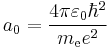 is the Bohr radius,
 are the generalized Laguerre polynomials of degree n − ℓ − 1.
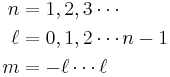
- n, m, ℓ are the principle, azimuthal , and magnetic quantum numbers respectively: which take the values:
NB: generalized Laguerre polynomials are defined differently by different authors - see main article on them and the Hydrogen atom.
Two-electron atoms or ions
The equation for any two-electron system, such as the neutral Helium atom (He, Z = 2), the negative Hydrogen ion (H–, Z = 1), or the positive Lithium ion (Li+, Z = 3) is: [48]

which simplifies to:
![E\psi = -\hbar^2\left[\frac{1}{2m_e}\left(\nabla_1^2 %2B\nabla_2^2 \right) %2B \frac{1}{Zm_p}\nabla_1\cdot\nabla_2\right] \psi %2B \frac{e^2}{4\pi\epsilon_0}\left[ \frac{1}{r_{12}^2} -Z\left( \frac{1}{r_1^2}%2B\frac{1}{r_2^2} \right) \right] \psi](/2012-wikipedia_en_all_nopic_01_2012/I/9bf4c5509b72783aaed5d18e9ad06d7a.png)
where r1 is the position of one electron (r1 = |r1| is its magnitude), r2 is the position of the other electron (r2 = |r2| is the magnitude), r12 = |r12| is the magnitude of the separation between them given by
mep is again the two-body reduced mass of an electron with respect to the nucleus, this time
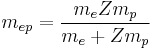
and Z is the atomic number for the element (not a quantum number).
The cross-term of two laplacians
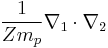
is known as the mass polarization term, which arises due to the motion of atomic nuclei. The wavefunction is a function of the two electron's positions:
There is no closed form solution to the equation for this equation.
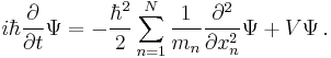
Time dependant
This is the equation of motion for the quantum state. In the most general form, it is written:[36]
Hamiltonians
Again, summarized below are the various forms the Hamiltonian takes, with the corresponding Schrödinger equations and forms of solutions.
| One particle | N particles | |
| One dimension | 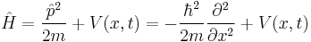 |
where the position of particle n is xn. |
 |
 |
|
 |
 |
|
| Three dimensions | 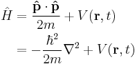 |
 |
 |
This last equation is in a very high dimension,[49] so the solutions are not easy to visualize. |
|
 |
 |
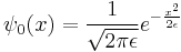
Gaussian wavepacket
The Gaussian wavepacket is: [50]
where a is a positive real number, the square of the width of the wavepacket.
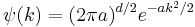
The Fourier transform
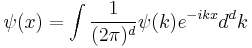
where d is the number of spatial dimensions, is a Gaussian again in terms of the wavenumber k:
Each separate wave only phase-rotates in time, so that the time dependent Fourier-transformed solution is:

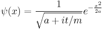
The inverse Fourier transform is still a Gaussian, but the parameter a has become complex, and there is an overall normalization factor.
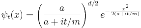
The branch of the square root is determined by continuity in time - it is the value which is nearest to the positive square root of a. It is convenient to rescale time to absorb m, replacing t/m by t.
The integral of ψ over all space is invariant, because it is the inner product of ψ with the state of zero energy, which is a wave with infinite wavelength, a constant function of space. For any energy state, with wavefunction η(x), the inner product:
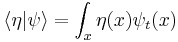 ,
,
only changes in time in a simple way: its phase rotates with a frequency determined by the energy of η. When η has zero energy, like the infinite wavelength wave, it doesn't change at all.
The quantity |ψ|2 is also invariant, which is a statement of the conservation of probability. Explicitly in one dimension:
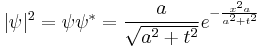
The width of the Gaussian is the interesting quantity, and it can be read off from the form of |ψ|2:
 .
.
The width eventually grows linearly in time, as  . This is wave-packet spreading, no matter how narrow the initial wavefunction, a Schrödinger wave eventually fills all of space. The linear growth is a reflection of the momentum uncertainty - the wavepacket is confined to a narrow width
  and so has a momentum which is uncertain by the reciprocal amount
  , a spread in velocity of
  , and therefore in the future position by
  , where the factor of m has been restored by undoing the earlier rescaling of time.
Nonlinear equation
The nonlinear Schrödinger equation is the partial differential equation (in dimensionless form)[51]
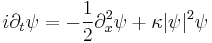
for the complex field ψ(x,t).
This equation arises from the Hamiltonian[51]
![H=\int \mathrm{d}x \left[{1\over 2}|\partial_x\psi|^2%2B{\kappa \over 2}|\psi|^4\right]](/2012-wikipedia_en_all_nopic_01_2012/I/e1b35484450918d6b846dd70d8cb6bf9.png)
with the Poisson brackets

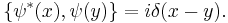
This is a classical field equation and, unlike its linear counterpart, it never describes the time evolution of a quantum state.
Relativistic generalizations
In order to extend Schrödinger's formalism to include relativity, the physical picture must be transformed. The Klein–Gordon equation
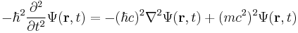
and the Dirac equation
are built from the relativistic mass–energy relation; so as a result these equations are relativistically invariant, and replace the Schrödinger equation in relativistic quantum mechanics. In fact the two equations are equivalent - in the sense that the Dirac equation is the "square root of" the Klein–Gordon equation.[34]
Solution methods
|
General techniques:
|
Methods for special cases: |
Free propagator
The narrow-width limit of the Gaussian wavepacket solution is the propagator K. For other differential equations, this is sometimes called the Green's function, but in quantum mechanics it is traditional to reserve the name Green's function for the time Fourier transform of K. When a is the infinitesimal quantity  , the Gaussian initial condition, rescaled so that its integral is one:
becomes a delta function, so that its time evolution:
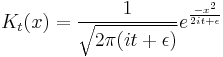
gives the propagator.
Note that a very narrow initial wavepacket instantly becomes infinitely wide, with a phase which is more rapidly oscillatory at large values of x. This might seem strange--- the solution goes from being concentrated at one point to being everywhere at all later times, but it is a reflection of the momentum uncertainty of a localized particle. Also note that the norm of the wavefunction is infinite, but this is also correct since the square of a delta function is divergent in the same way.
The factor of is an infinitesimal quantity which is there to make sure that integrals over K are well defined. In the limit that becomes zero, K becomes purely oscillatory and integrals of K are not absolutely convergent. In the remainder of this section, it will be set to zero, but in order for all the integrations over intermediate states to be well defined, the limit  is to only to be taken after the final state is calculated.
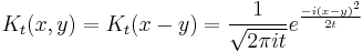
The propagator is the amplitude for reaching point x at time t, when starting at the origin, x=0. By translation invariance, the amplitude for reaching a point x when starting at point y is the same function, only translated:
In the limit when t is small, the propagator converges to a delta function:
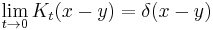
but only in the sense of distributions. The integral of this quantity multiplied by an arbitrary differentiable test function gives the value of the test function at zero. To see this, note that the integral over all space of K is equal to 1 at all times:
since this integral is the inner-product of K with the uniform wavefunction. But the phase factor in the exponent has a nonzero spatial derivative everywhere except at the origin, and so when the time is small there are fast phase cancellations at all but one point. This is rigorously true when the limit  is taken after everything else.
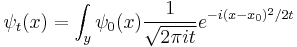
So the propagation kernel is the future time evolution of a delta function, and it is continuous in a sense, it converges to the initial delta function at small times. If the initial wavefunction is an infinitely narrow spike at position  :
:
it becomes the oscillatory wave:
Since every function can be written as a sum of narrow spikes:
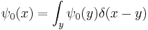
the time evolution of every function is determined by the propagation kernel:
And this is an alternate way to express the general solution. The interpretation of this expression is that the amplitude for a particle to be found at point x at time t is the amplitude that it started at times the amplitude that it went from to x, summed over all the possible starting points. In other words, it is a convolution of the kernel K with the initial condition.
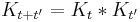
Since the amplitude to travel from x to y after a time  can be considered in two steps, the propagator obeys the identity:
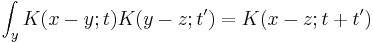
Which can be interpreted as follows: the amplitude to travel from x to z in time t+t' is the sum of the amplitude to travel from x to y in time t multiplied by the amplitude to travel from y to z in time t', summed over all possible intermediate states y. This is a property of an arbitrary quantum system, and by subdividing the time into many segments, it allows the time evolution to be expressed as a path integral.
Analytic continuation to diffusion
The spreading of wavepackets in quantum mechanics is directly related to the spreading of probability densities in diffusion. For a particle which is random walking, the probability density function at any point satisfies the diffusion equation:
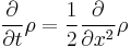
where the factor of 2, which can be removed by a rescaling either time or space, is only for convenience.
A solution of this equation is the spreading gaussian:
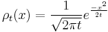
and since the integral of  , is constant, while the width is becoming narrow at small times, this function approaches a delta function at t=0:
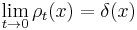
again, only in the sense of distributions, so that
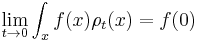
for any smooth test function f.
The spreading Gaussian is the propagation kernel for the diffusion equation and it obeys the convolution identity:
Which allows diffusion to be expressed as a path integral. The propagator is the exponential of an operator H:
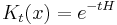
which is the infinitesimal diffusion operator.

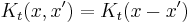
A matrix has two indices, which in continuous space makes it a function of x and x'. In this case, because of translation invariance, the matrix element K only depend on the difference of the position, and a convenient abuse of notation is to refer to the operator, the matrix elements, and the function of the difference by the same name:
Translation invariance means that continuous matrix multiplication:
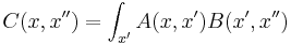
is really convolution:

The exponential can be defined over a range of t's which include complex values, so long as integrals over the propagation kernel stay convergent.
As long as the real part of z is positive, for large values of x K is exponentially decreasing and integrals over K are absolutely convergent.
The limit of this expression for z coming close to the pure imaginary axis is the Schrödinger propagator:
and this gives a more conceptual explanation for the time evolution of Gaussians. From the fundamental identity of exponentiation, or path integration:
holds for all complex z values where the integrals are absolutely convergent so that the operators are well defined.
So that quantum evolution starting from a Gaussian, which is the diffusion kernel K:

gives the time evolved state:
This explains the diffusive form of the Gaussian solutions:
See also
- Basic concepts of quantum mechanics
- Dirac equation
- P-adic quantum mechanics
- Quantum chaos
- Quantum number
- Relation between Schrödinger's equation and the path integral formulation of quantum mechanics
- Schrödinger's cat
- Schrödinger field
- Schrödinger picture
- Theoretical and experimental justification for the Schrödinger equation
Notes
- ^ Schrödinger, E. (1926). "An Undulatory Theory of the Mechanics of Atoms and Molecules". Physical Review 28 (6): 1049–1070. Bibcode 1926PhRv...28.1049S. doi:10.1103/PhysRev.28.1049. Archived from the original on 2008-12-17. http://web.archive.org/web/20081217040121/http://home.tiscali.nl/physis/HistoricPaper/Schroedinger/Schroedinger1926c.pdf.
- ^ The New Quantum Universe, T.Hey, P.Walters, Cambridge University Press, 2009, ISBN 978-0-521-56457-2
- ^ Shankar, R. (1994). Principles of Quantum Mechanics (2nd ed.). Kluwer Academic/Plenum Publishers. p. 143. ISBN 978-0-306-44790-7.
- ^ de Broglie, L. (1925). "Recherches sur la théorie des quanta [On the Theory of Quanta]". Annales de Physique 10 (3): 22–128. http://tel.archives-ouvertes.fr/docs/00/04/70/78/PDF/tel-00006807.pdf. Translated version.
- ^ Schrodinger, E. (1984). Collected papers. Friedrich Vieweg und Sohn. ISBN 3700105738. See introduction to first 1926 paper.
- ^ a b Encyclopaedia of Physics (2nd Edition), R.G. Lerner, G.L. Trigg, VHC publishers, 1991, (Verlagsgesellschaft) 3-527-26954-1, (VHC Inc.) 0-89573-752-3
- ^ Erwin Schrödinger, "The Present situation in Quantum Mechanics," p. 9 of 22. The English version was translated by John D. Trimmer. The translation first appeared first in in Proceedings of the American Philosophical Society, 124, 323-38. It later appeared as Section I.11 of Part I of Quantum Theory and Measurement by J.A. Wheeler and W.H. Zurek, eds., Princeton University Press, New Jersey 1983).
- ^ Sommerfeld, A. (1919). Atombau und Spektrallinien. Braunschweig: Friedrich Vieweg und Sohn. ISBN 3871444847.
- ^ For an English source, see Haar, T.. The Old Quantum Theory.
- ^ Rhodes, R. (1986). Making of the Atomic Bomb. Touchstone. ISBN 0-671-44133-7.
- ^ Schrödinger, E. (1926). "Quantisierung als Eigenwertproblem; von Erwin Schrödinger". Annalen der Physik, (Leipzig): 361–377. http://gallica.bnf.fr/ark:/12148/bpt6k153811.image.langFR.f373.pagination.
- ^ Einstein, A.; et. al.. Letters on Wave Mechanics: Schrodinger-Planck-Einstein-Lorentz.
- ^ Moore, W.J. (1992). Schrödinger: Life and Thought. Cambridge University Press. p. 219. ISBN 0-521-43767-9.
- ^ Moore, W.J. (1992). Schrödinger: Life and Thought. Cambridge University Press. p. 220. ISBN 0-521-43767-9.
- ^ It is clear that even in his last year of life, as shown in a letter to Max Born, that Schrödinger never accepted the Copenhagen interpretation (cf. p. 220). Moore, W.J. (1992). Schrödinger: Life and Thought. Cambridge University Press. p. 479. ISBN 0-521-43767-9.
- ^ Quanta: A handbook of concepts, P.W. Atkins, Oxford University Press, 1974, ISBN 0-19-855493-1
- ^ Physics of Atoms and Molecules, B.H. Bransden, C.J.Joachain, Longman, 1983, ISBN 0-582-44401-2
- ^ a b Quantum Physics of Atoms, Molecules, Solids, Nuclei and Particles (2nd Edition), R. Resnick, R. Eisberg, John Wiley & Sons, 1985, ISBN 978-0-471-873730
- ^ Quanta: A handbook of concepts, P.W. Atkins, Oxford University Press, 1974, ISBN 0-19-855493-1
- ^ Feynman Lectures on Physics (Vol. 3), R. Feynman, R.B. Leighton, M. Sands, Addison-Wesley, 1965, ISBN 0-201-02118-8
- ^ Electromagnetism (2nd edition), I.S. Grant, W.R. Phillips, Manchester Physics Series, 2008 ISBN 0 471 92712 0
- ^ The New Quantum Universe, T.Hey, P.Walters, Cambridge University Press, 2009, ISBN 978-0-521-56457-2
- ^ http://arxiv.org/abs/hep-ph/0301145
- ^ http://physicsworld.com/cws/article/news/3525
- ^ Quantum Mechanics Demystified, D. McMahon, Mc Graw Hill (USA), 2006, ISBN(10) 0 07 145546 9
- ^ Quantum Mechanics Demystified, D. McMahon, Mc Graw Hill (USA), 2006, ISBN(10) 0 07 145546 9
- ^ Quantum Mechanics, E. Abers, Pearson Ed., Addision Wesley, Prentice Hall Inc, 2004, ISBN 9780131461000
- ^ Quantum Mechanics, E. Abers, Pearson Ed., Addision Wesley, Prentice Hall Inc, 2004, ISBN 9780131461000
- ^ Encyclopaedia of Physics (2nd Edition), R.G. Lerner, G.L. Trigg, VHC publishers, 1991, (Verlagsgesellschaft) 3-527-26954-1, (VHC Inc.) 0-89573-752-3
- ^ Quantum Mechanics, E. Abers, Pearson Ed., Addision Wesley, Prentice Hall Inc, 2004, ISBN 9780131461000
- ^ Physics of Atoms and Molecules, B.H. Bransden, C.J.Joachain, Longman, 1983, ISBN 0-582-44401-2
- ^ Quantum Mechanics, E. Abers, Pearson Ed., Addision Wesley, Prentice Hall Inc, 2004, ISBN 9780131461000
- ^ Quantum Mechanics, E. Abers, Pearson Ed., Addision Wesley, Prentice Hall Inc, 2004, ISBN 9780131461000
- ^ a b Quantum Field Theory, D. McMahon, Mc Graw Hill (USA), 2008, ISBN 978-0-07-154382-8
- ^ van Oosten, A. B. (2006). "Covariance of the Schrödinger equation under low velocity boost". Apeiro 13 (2): 449–454.
- ^ a b Shankar, R. (1994). Principles of Quantum Mechanics. Kluwer Academic/Plenum Publishers. pp. 143ff. ISBN 978-0-306-44790-7.
- ^ Quantum Mechanics Demystified, D. McMahon, Mc Graw Hill (USA), 2006, ISBN(10) 0 07 145546 9
- ^ Feynman, R.P.; Leighton, R.B.; Sand, M. (1964). "Operators". The Feynman Lectures on Physics. 3. Addison-Wesley. pp. 20–7. ISBN 0201021153.
- ^ Shankar, R. (1994). Principles of Quantum Mechanics. Kluwer Academic/Plenum Publishers. pp. 151ff. ISBN 978-0-306-44790-7.
- ^ Quantum Mechanics Demystified, D. McMahon, Mc Graw Hill (USA), 2006, ISBN(10) 0 07 145546 9
- ^ Physical chemistry, P.W. Atkins, Oxford University Press, 1978, ISBN 0 19 855148 7
- ^ Solid State Physics (2nd Edition), J.R. Hook, H.E. Hall, Manchester Physics Series, John Wiley & Sons, 2010, ISBN 978 0 471 92804 1
- ^ Quanta: A handbook of concepts, P.W. Atkins, Oxford University Press, 1974, ISBN 0-19-855493-1
- ^ Molecular Quantum Mechanics Parts I and II: An Introduction to QUANTUM CHEMISRTY (Volume 1), P.W. Atkins, Oxford University Press, 1977, ISBN 0-19-855129-0
- ^ http://hyperphysics.phy-astr.gsu.edu/hbase/hframe.html
- ^ Physics for Scientists and Engineers - with Modern Physics (6th Edition), P. A. Tipler, G. Mosca, Freeman, 2008, ISBN 0 7167 8964 7
- ^ David Griffiths (2008). Introduction to elementary particles. Wiley-VCH. pp. 162–. ISBN 9783527406012. http://books.google.com/books?id=w9Dz56myXm8C&pg=PA162. Retrieved 27 June 2011.
- ^ Physics of Atoms and Molecules, B.H. Bransden, C.J.Joachain, Longman, 1983, ISBN 0-582-44401-2
- ^ Shankar, R. (1994). Principles of Quantum Mechanics. Kluwer Academic/Plenum Publishers. p. 141. ISBN 978-0-306-44790-7.
- ^ Quantum Mechanics, E. Abers, Pearson Ed., Addision Wesley, Prentice Hall Inc, 2004, ISBN 9780131461000
- ^ a b V.E. Zakharov; S.V. Manakov (1974). "On the complete integrability of a nonlinear Schrödinger equation". Journal of Theoretical and Mathematical Physics 19 (3): 551–559. Bibcode 1974TMP....19..551Z. doi:10.1007/BF01035568. Originally in: Teoreticheskaya i Matematicheskaya Fizika 19 (3): 332–343. June, 1974
References
- Paul Adrien Maurice Dirac (1958). The Principles of Quantum Mechanics (4th ed.). Oxford University Press.
- David J. Griffiths (2004). Introduction to Quantum Mechanics (2nd ed.). Benjamin Cummings. ISBN 0131244051.
- Richard Liboff (2002). Introductory Quantum Mechanics (4th ed.). Addison Wesley. ISBN 0805387145.
- David Halliday (2007). Fundamentals of Physics (8th ed.). Wiley. ISBN 0471159506.
- Serway, Moses, and Moyer (2004). Modern Physics (3rd ed.). Brooks Cole. ISBN 0534493408.
- Walter John Moore (1992). Schrödinger: Life and Thought. Cambridge University Press. ISBN 0521437679.
- Schrödinger, Erwin (December 1926). "An Undulatory Theory of the Mechanics of Atoms and Molecules". Phys. Rev. 28 (6) 28 (6): 1049–1070. Bibcode 1926PhRv...28.1049S. doi:10.1103/PhysRev.28.1049.
External links
- Quantum Physics - textbook with a treatment of the time-independent Schrödinger equation
- Linear Schrödinger Equation at EqWorld: The World of Mathematical Equations.
- Nonlinear Schrödinger Equation at EqWorld: The World of Mathematical Equations.
- The Schrödinger Equation in One Dimension as well as the directory of the book.
- All about 3D Schrödinger Equation
- Mathematical aspects of Schrödinger equations are discussed on the Dispersive PDE Wiki.
- Web-Schrödinger: Interactive solution of the 2D time dependent Schrödinger equation
- An alternate derivation of the Schrödinger Equation
- Online software-Periodic Potential Lab Solves the time independent Schrödinger equation for arbitrary periodic potentials.